Visualizing a simple GW chirp signal

The gravitational waveform from inspiralling binaries is known as a chirp waveform. The amplitude and the frequency of the waveform increases with time and hence it is called a chirp (similar to a bird’s chirp). Here I’ll go through the steps to compute a simple waveform for inspiralling binaries in Python.

Setup

I will be using Numpy for calculations, Matplotlib for plotting and Astropy for using some constants (like $c, G$). You can install these packages using pip by clicking the link below. (Note that Astropy can be avoided for this exercise and the constant values can be hardcoded directly.)

• Numpy installation
• Matplotlib installation
• Astropy installation

import numpy as np
import matplotlib.pyplot as plt
from astropy import constants as const

Using the constants module we will define the constants reuired for this computation

G = const.G.value #gravitational constant
c = const.c.value #speed of light
Msun = const.M_sun.value  #Mass of Sun
pc = const.pc.value #parsec
Mpc = 10**6 * pc 

Frequency evolution

Now that we have the setup ready, we will look at the frequency evolution ($f$ vs $t$) for the waveform. From the theory of inspiralling binaries emiting GWs (I’m making a series of posts on that too!) we get $\dot{f}$ as,

where the chirp mass $M_c$ is given by $\frac{(m1 \ m2)^{3/5}}{(m_1 + m_2)^{1/5}}$. This equation can then be integrated to get $t(f)$ :

\(t = t_c - \frac{3}{256} \Bigl( \frac{c^3}{G M_c}\Bigr)^{5/3} (\pi f)^{-8/3}\) Here $t_c$ denotes the time of coalescence and it is completely arbitary (We’ll take $t_c = 0$). The equation tells us how close we are to the merger time. This can be now coded u

  #chirp mass
  def Mchirp(m1,m2):
    return (m1*m2)**(3/5) * (m1+m2)**(-1/5)

  #parameters
  m1 = 30 * Msun
  m2 = 30 * Msun
  Mc = Mchirp(m1,m2)
  D = 1*Mpc

  f0 = 10 #starting frequency
  freq = np.linspace(f0,50,100)
  tc = 0.0 #merger time (s)

  def tau(f,Mc):
    return (3/156) * (c**3/(G*Mc))**(5/3) * (np.pi * f)**(-8/3)4

  time = tc - tau(freq,Mc)

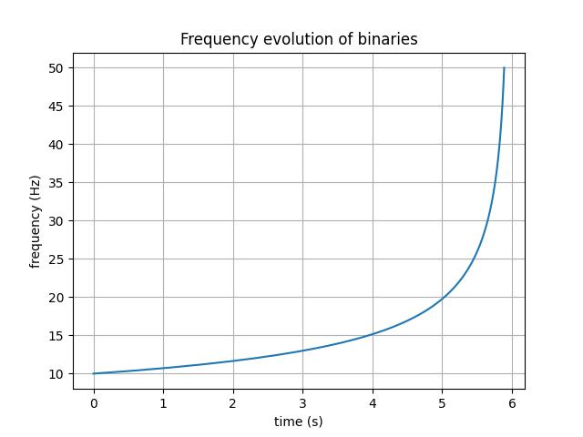
We can now plot $f$ vs $t$ and compare it with the kind of behaviour that you expect from a gravitational waveform.

tduration = time[-1] - time[0] #duration of the signal
torder = time - time[0] #rearranging the time array such that the t0 = 0 and merger time is tduration

plt.figure()
plt.xlabel("time (s)")
plt.ylabel("frequency (Hz)")
plt.title("Frequency evolution of binaries")
plt.grid()

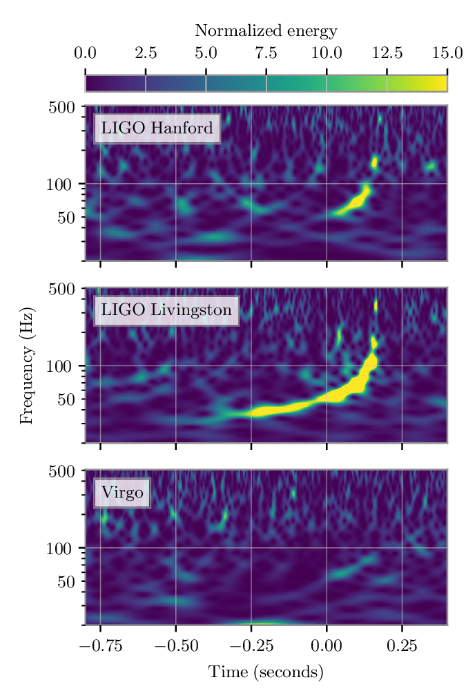
This is similar to the Time–frequency plots that we usualy plot for a detection like the one below for GW190412. The frequency is expected to increase as the GWs are emitted away, the orbital frequency increases.

The Chirp Signal

Now that we have plotted the time-frequency plot, the next step would be to visualise the chirp signal. The waveform is define by

1. Amplitude :

1. Phase:

$\dot{f}$ is defined above and $\phi_{0}$ is the initial phase of the binary. The waveform is then

Now for plotting, we will use the above frequency series and using the $t(f)$ we can calculate $t$ which then can be used to compute $\phi(t)$ and in turn $h(t)$.

def h(Mc,D,f):
    
    #Amplitude
    h0 = 4*G*c**(-2)*Mc/D * (G*c**(-3) * np.pi * f*Mc)**(2/3)
    fdot = dfdt(f,Mc)
    t = tc - tau(f,Mc)
    
    #phase
    phi = 2*np.pi*f*t + np.pi*fdot*t**2+phi0
    
    return (t,h0*np.cos(phi))

freq = np.linspace(f0,100,5000)


t,hstrain = h(Mc,D,freq)
plt.figure()
plt.plot(t-t[0],hstrain)
plt.grid()
plt.xlabel("time(s)")
plt.ylabel("h(t)")
plt.title("A simple chirp signal")

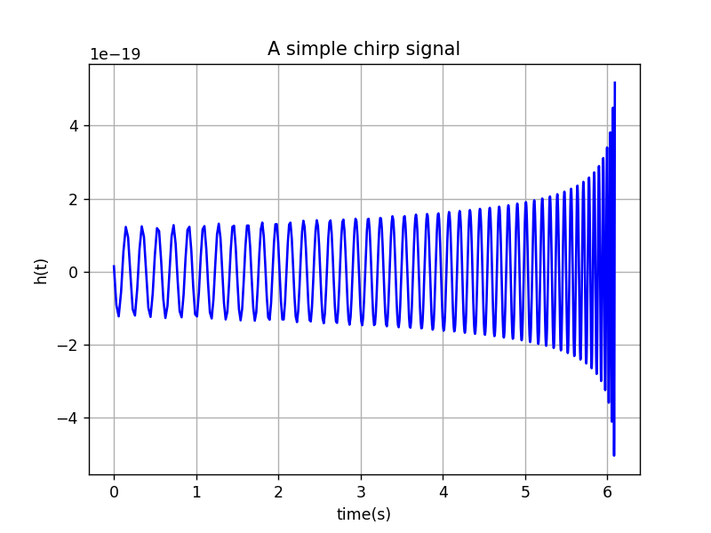
This is a simple chirp waveform that we have computed. As you can see the amplitude and the frequency of the waveform increases with time.